Our data is now sufficiently clean, and we now want to divide up the data into sections of interest to us. In this experiment, we are looking at brain data for when an individual looked at images to-be-remembered under two conditions - during rhythmic presentation and arrhythmic presentation. Based on the behavioural data (Jones & Ward (2019)) we know that those images that were presented rhythmically to participants were better remembered than those that were presented arrhythmically. Now we want to carve up the brain data to examine what were the differences in the brain when these images were being encoded. Brain data here, and EEG specifically, is particularly useful as during the encoding of images we require no behavioural output from the participant - that means that we can’t look at behaviour to make an inference about underlying cognitive processes. However, the EEG data here may provide us with some insight when comparing conditions.
As well as carving up the continuous data around the events of interest, we are also going to ‘baseline correct.’ Baseline correction is effectively a simple correction of EEG data to, usually, the pre-stimulus interval. Specifically, EEG data before the event of interest is assumed to have a mean of zero voltage and the EEG activity is simply shifted in the voltage domain to meet this assumption.
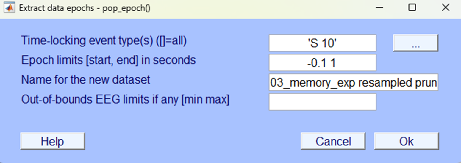
We will now carve up the continuous EEG data around ‘triggers’ that correspond to the presentation of images to-be-remembered under both conditions. Specifically, we will carve up the brain data 100ms before the image appears and 1000ms after it is on the screen. The two triggers that correspond to the presentation of images under different conditions are S 10 which corresponds to the rhythmic condition and S 12 which corresponds to the arrhythmic condition. We’ll carve up the EEG separately for each condition.
Again, EEG terms can be a little confusing two words are often used to mean the same thing:
- Epoch
- Segment
Both usually refer to a small section of the EEG data usually around a specific event - a stimulus or response.
How
Segment
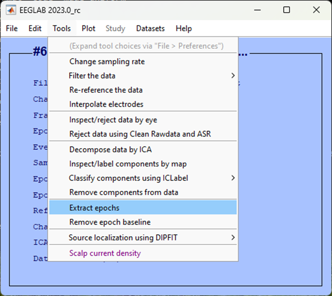
EEGLAB allows you to segment the data using the following tool:
-> Tools
  -> Extract epochs
In the next pop-up window, we want to specify the events, we’ll first lock to the presentation of images during the rhythmic condition so click on the three dots ... and select the trigger S 10. We want to specify 100 ms before the image and up to one second after as our epoch. To do so, in the Epoch limits [start, end] in seconds enter -0.1 1.
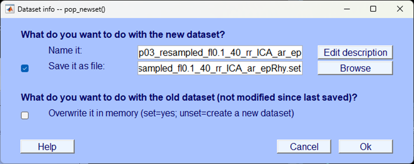
In the next pop-up save it so you can identify the dataset as one that is segmented specifically for the rhythmic condition.
Baseline correct
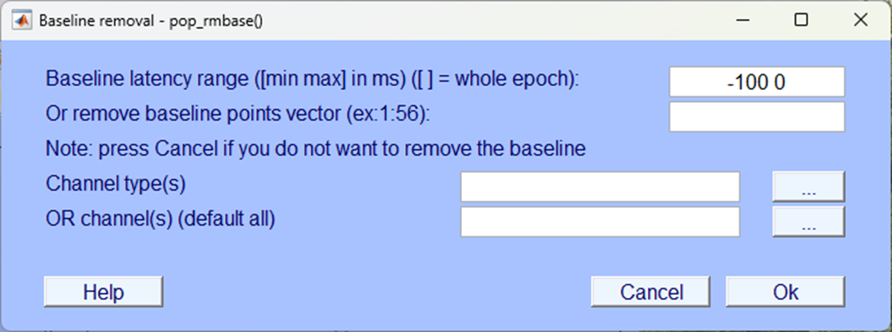
We next need to correct the segmented data such that it is relative to a pre-stimulus baseline.
-> Tools
  -> Remove epoch baseline
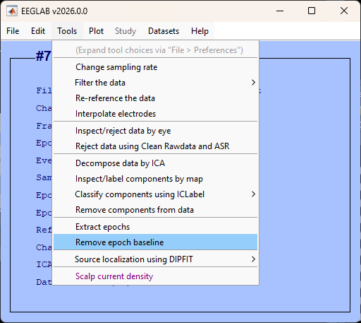
An pop-up will prompt you to baseline correct, the default should use the pre-stimulus period as a baseline and this is what we want so you can simply accept by clicking Ok.
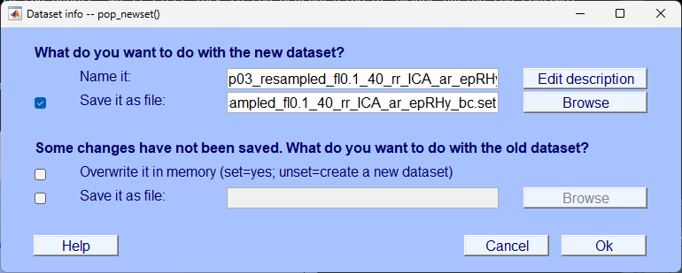
You’ll be prompted again to save the data after baseline correcting, you can add the suffix _bc for ‘baseline correct’ and save.
Plot the data
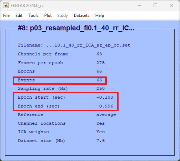
You can now see in the EEGLAB home window that the dataset consisted of segmented data with an epoch that starts at -100 ms from the event and ends just before 1000 ms. Further, there are far fewer events in the data file as we’ve selected only those relevant to this condition.
If we plot the data, we can see it is no longer continuous, click:
-> Plot
  -> Channel data (scroll)
You should see something quite different to what you’ve seen before using this function, a little like what’s below.
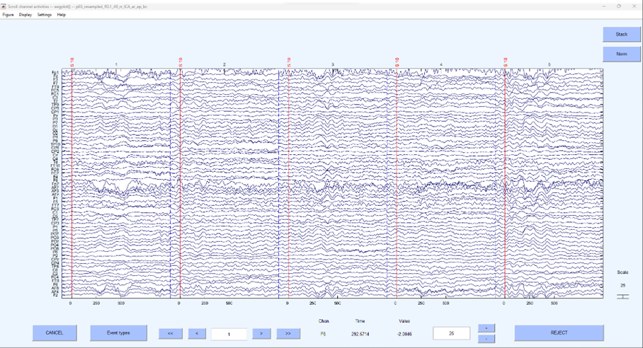
This is no longer continuous data but rather the segments around the specific even of interest that have been stitched together. To generate an ERP, we can average across each segment and plot the average, this is simple enough to do in EEGLAB, click:
-> Plot
   -> Channel ERPs
     -> In scalp/rect. array
Accept the defaults in the pop-up window and click Ok.

You should now be looking at an ‘Event Related Potential’ or ‘ERP’ - all activity within one condition, averaged over repeated trials and centred around an event. You should have one plot for each electrode and the electrodes are plotted where they appear on a topographical representation of the scalp.
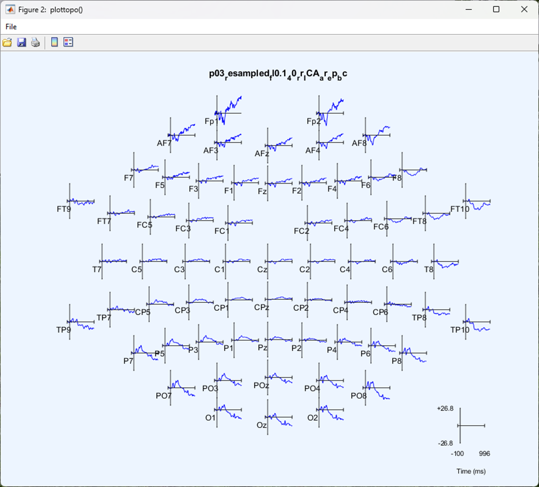
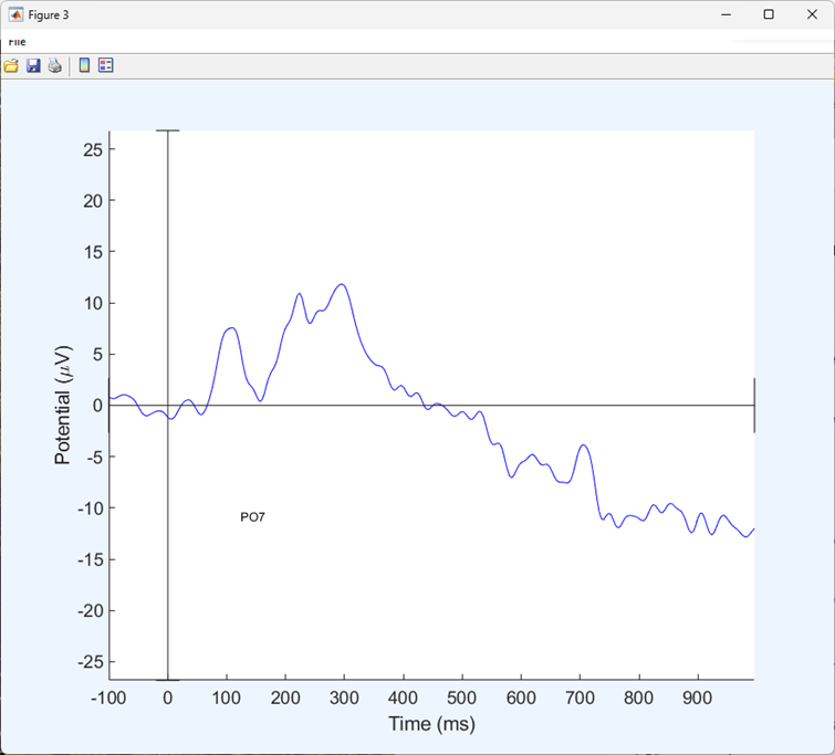
You can click on any electrode for a closer look at the ERP for that electrode.
Segment the next condition
We now want to extract the data averaged around the ‘arrhythmic’ condition. To do this we need to load a dataset before we run the segmentation procedure, in our case we labelled the file P03_resampled_fl0.1_40_rr_ICA_ar, click:
-> File
  -> Load existing dataset
Select your file that has been resampled, filtered, interpolated (if needed), re-referenced, ICA blink reduction and artefact rejected.
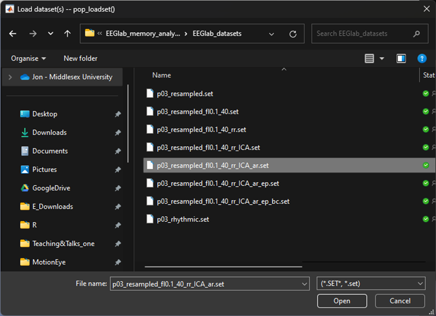
Once you’ve loaded the file - we want to segment based on the arrhythmic condition. To do so follow through the previous steps in this chapter from Segment. But this time, segment around the trigger S 12.
When you are segmenting the data, it’s important you remember that you need to do so twice for each participant, remember the trigger codes:
S 10 = Rhythmic condition
S 12 = Arrhythmic condition
Question 1 | In EEG analysis, what’s another word for ‘segment’?
Question 2 | What is EEG activity that shifts to a mean of zero during baseline correction?